


In custody transfer applications where the buying and selling of commodities like natural gas is involved, calibration checks are performed frequently as a matter of fiduciary responsibility. For the purpose of this application note, the use of gas custody transfer flow computers in the natural gas transmission industry is referenced. Flow computers need multiple measurements to calibrate each device. In the normal application, three measurements are made: volumetric flow, static (line) pressure and temperature. A calculation is performed using this data to determine the actual mass of the gas flowing through the pipeline.

The Fluke 721 Precision Pressure Calibrator has special features that support the complete calibration of natural gas multi-variable electronic flowmeters and other types of flow computers. With two internal pressure ranges, external Fluke 750P pressure modules and an optional precision RTD probe, all of the calibrations required for the flow computer can be performed with just one instrument. The Fluke 721 is available with two built-in pressure ranges from from 16 psi/1 bar up to 5000 psi/345 bar. For this application, the configuration with the low pressure sensor (P1) 16 psi/1 bar and high pressure sensor (P2) of 1500 psi/100 bar is frequently the best fit. Since the Fluke 721 has an accuracy specification as a percent of full scale, it is important to closely match the full scale of the calibrator to the scale of the application in order to get the best performance. (See sidebar on system accuracy calculation and importance of maintaining an adequate accuracy ratio). In addition to the calibrator itself, a high and low pressure calibration pressure source will be needed. An accessory RTD probe is also required for measuring temperature. An appropriate low pressure source with 0.01 inH2O of resolution is needed for the low pressure test, and a high pressure source such as a regulated nitrogen bottle or hydraulic hand pump are required. One pump style typically does not work well for both tests or extensive cleaning is required to switch from hydraulic (oil or water) to pneumatic testing. High pressure pumps typically do not have the desired resolution for the low pressure test.
Gas custody transfer flow computer operational theory
Custody transfer flow computers are called by a variety of names including electronic flowmeters (EFMs) and multi-variable flow computers, but they all feature some common principles of operation.
- Volumetric flow measurement uses some type of flow restriction such as an orifice plate to generate a pressure drop. The differential pressure created across this pressure drop is measured by the flow computer as the primary measurement. It is based on the principle that flow velocity is proportional to the square root of the pressure drop. The volumetric rate is then calculated from the velocity by knowing the diameter of the pipe in which the gas is flowing.
The measured pressure drop (differential) is typically around 200 inches of water column (“WC) or 8-10 psi. - To convert volumetric flow to mass flow you also need to know the density of the mass per volume of the flowing media. The flow computer makes this calculation using 2 additional measurements, plus a range of factors/constants based on the flowing media. The two additional measurements are the static pressure of the gas in the pipeline and the temperature of the gas in the pipeline.
The static pressure in these applications ranges widely from a low of about 300 psi / 20 bar to a high of about 2000 psi / 138 bar.
The temperature of the gas is usually at ambient, so it is within the range of normal environmental conditions. - A final consideration about flow computers is how they are typically installed and used.
Industrial applications use either the analog output of the flowmeter (4 to 20 mA) or a digital output like the HART signal to get data from the flowmeter to a control system or data acquisition system.
This analog output is generally not used in gas pipeline applications. Instead, the flowmeter is a specialized device that operates standalone to measure and record the total mass flow through the pipeline. The total is periodically “downloaded” from the flowmeter to be used in an accounting of gas flow and custody transfer.
This information is also often sent through wirelessly to a central control point in operations.
The flowmeter may be packaged with other electronic devices to be able to perform this function or it may be purpose manufactured, which is the most common type.
System Accuracy Determination
In order to effectively calibrate an instrument, the calibrator used must be more accurate than the instrument by some factor. The factor will vary according to the application, but it should be as large as is practical. The minimum factor is generally considered to be 3 to 4 times. The common term for expressing this factor is Test Uncertainty
Ratio or TUR. If the calibrator is 4 times more accurate than the device being tested it is referred to as having a TUR of 4:1. The rationale behind this comes from a technique for the statistical analysis of the error in a system. This technique is called Root Square Sum or RSS. To determine the error in a system you take the square root of the sum of the errors squared for all elements in the system. Note that this is not the maximum possible error in a system, but is the largest error which is statistically likely. This formula describes the calculation, where Et is the total error and E1, etc. are the errors of the individual components of the system.

By using a TUR of 4:1, the effect of the error in the calibrator is reduced to a small percentage of the error of the instrument under test and can therefore generally be disregarded. As an alternative to having a calibrator with the appropriate ratio, users may elect to de-rate the performance of the instrument to a value four times that of the calibrator.
For example, using a calibrator with ±0.05% accuracy would have a TUR of 4:1 testing an instrument with an accuracy of ±0.2%. Due to the continual advances in instrument technology, calibration technology may, from time to time, fail to provide the necessary TUR to calibrate to the instrument manufacturer’s rated specification. Alternately you can tighten the test tolerance to 80% of the desired specification to gain the same confidence using a technique called guardbanding. The fundamental concept of guardbanding is to restrict the Pass/Fail limits applied to a calibration test based on a defined criterion. The purpose of guardbanding is to control the risk of accepting an out-of-tolerance unit, or rejecting an in-tolerance unit. Without guardbanding the result of a test will be Pass or Fail. With guardbanding the result of a test will be Pass, Fail, or Indeterminate. A Pass or Fail test result without guardbanding may change to a result of Indeterminate with guardbanding. For more information on guardbanding refer to the application note “Guardbanding with Confidence” at www.fluke.com/guardbanding.
How to calibrate the flow computer
Each flow computer manufacturer has created a proprietary method of calibration, but they all use the same general technique, which will be described here.
In these proprietary calibrations, the manufacturer has provided a software application, which runs on a notebook computer (PC). The PC is connected to the serial port or USB port of the flow computer. In this way, the software both instructs the user to connect appropriate signals to the flow computer (either pressure or temperature) and communicates that information to the flow computer so that calibration errors can be corrected.
Note: This procedure is a generic description of the calibration process using the Fluke-721-1615 as an example. The actual procedure will vary based on the original equipment manufacturer’s design and instructions, test equipment used and on local process and policy.
Detailed Procedure
- Setup
a. Turn on the calibrator and make sure that you see three measurements, usually [P1], [P2], and [RTD]. If you only see two measurements, press F1 [P1/P2] until three measurements appear. If you see three measurements, but not [RTD], press F2 [mA/V/RTD] until [RTD] appears. Refer to the user guide for more information about calibrator setups.
b. If needed, set the upper display (P1) to use inches of water column (in H2O 60°F) as the engineering unit, the middle display (p2) to use psi as the engineering unit and the bottom display (RTD) to use °F as the engineering unit. Refer to the user guide for more information about setting engineering units.
Note: Once the calibrator has been configured to use these settings, they become the default unless subsequently changed by the user.
c. If necessary, zero both pressure displays while vented to atmosphere. Refer to the user guide for information about zeroing the pressure displays.
d. Isolate the flow computer from the process. (It is normally installed with a 5 valve manifold. Closing the valves on the process side of the manifold will isolate it from the process). Be sure to follow local policy and procedure when performing this step. - Differential pressure calibration
a. The differential pressure calibration is performed using atmospheric pressure as a reference, so the low pressure connection of the flow computer or pressure transmitter is vented and the high pressure connection on the flow computer or transmitter is connected to the low pressure port on the calibrator.
b. Connect the notebook computer (PC) to the flow computer serial or USB port. Use the PC to initiate the calibration process.
c. The PC will instruct the user to apply one or more test pressures to the flow computer or transmitter. For example, on a device with a full scale differential measurement of 200” WC, the test pressures may be 0, 100 and 200” WC. In each case, it is not necessary to provide the exact pressure called for since the user will also be prompted to enter the actual pressure applied at each test point.
d. Set the hand pump pressure/vacuum control to the pressure mode and close the vent valve. Squeeze the pump handles until the desired pressure is generated. The vernier or fine pressure control of the pump can be used to adjust the pressure up or down in small amounts.
Note: 200” WC is approximately 7.2 psi. Since the pump can easily exceed this pressure, it may be best to apply repeated short squeezes of the pump to allow for better control. The rate of pressure increase will be affected by the volume of the test system with faster increases when the volume is lower. - Static pressure calibration
a. For the static pressure calibration, the test pressure will normally be applied to either the same high pressure port or both the high and low pressure ports simultaneously. Refer to the manufacturer’s instructions for details on the exact method of connection to perform this test. Connect the high pressure sensor input (p2) to the appropriate port on the flow computer or transmitter and to the high pressure test source such as hand pump or nitrogen bottle.
Note: if the source has 2 ports, one can be connected to the (p2) input and the other to the port on the flow computer/transmitter.
b. The PC will instruct the user to apply one or more test pressures to the flow computer/ transmitter. For example, on a device with a full scale static pressure measurement of 1500 psi, the test pressures may be 0, 750 and 1500 psi. In each case, it is not necessary to provide the exact pressure called for since the user will be prompted to enter the actual pressure applied at each test point.
c. Use the high pressure test source to generate the called for pressures and enter observed data when prompted.
d. Set the hand pump pressure/vacuum control to the pressure mode and close the vent valve. Squeeze the pump handles until the desired pressure is generated. The vernier or fine pressure control of the pump can be used to adjust the pressure up or down in small amounts.
Note: 200” WC is approximately 7.2 psi. Since the pump can easily exceed this pressure, it may be best to apply repeated short squeezes of the pump to allow for better control. The rate of pressure increase will be affected by the volume of the test system with faster increases when the volume is lower.
e. When the differential calibration is complete, open the pump vent control and disconnect the calibrator from the flow computer or transmitter. - Temperature calibration
a. Calibration of the temperature measurement on the flow computer is done with a single temperature point at the pipeline operating temperature.
b. A test thermowell is provided adjacent to the in service measuring RTD connected to the flow computer or temperature transmitter. Insert the calibrator probe into the test thermowell and allow time for the measurement to reach a stable value.
Note: Inserting the probe can be done prior to the pressure calibrations if local conditions permit. That allows sufficient time to reach stability.
c. This calibration is based on the concept that the same temperature is measured at both thermowells and, therefore, the measured values should be identical. The PC will prompt the user to enter the value observed on the calibrator.
d. Remove the RTD from the test thermowell. The calibration is complete. - Wrap up
a. Follow local policy and procedures and manufacturer’s instructions for returning the flow computer to service.
b. If the flow computer has transmitters for measurement of differential pressure, static pressure and temperature the flow computer interprets the transmitters scaled mA output via its mA analog inputs. In this instance, if the calibration is unsuccessful, the individual transmitters may need calibration and adjustment to remove errors. One last source of errors to consider in this configuration, which, is often overlooked is the mA input A/D of the flow computer which typically has an offset and gain adjustment.